Tutorial 1: parameter estimation and sensitivity analysis

This tutorial shows you how to build computational models, estimate parameter values from experimental data, and identify sensitive components in complex biochemical systems. We will use a mechanistic model of the c-Fos expression network dynamics [Nakakuki et al., 2010]. For a detailed description of the model, please refer to the following paper:

Nakakuki, T. et al. Ligand-specific c-Fos expression emerges from the spatiotemporal control of ErbB network dynamics. Cell 141, 884–896 (2010). https://doi.org/10.1016/j.cell.2010.03.054

Requirements

biomass>=0.8.0 for simulation, parameterization, and analysis of the model
tqdm for visualizing progress bars

To check the software versions, run the following code:

import biomass
print('biomass version:', biomass.__version__)

Model preparation

A brief description of each file/folder is below:

Name	Content
`name2idx/`	Names of model parameters and species
`reaction_network.py`	Flux vector and reaction indices grouped according to biological processes
`ode.py`	Differential equation, parameters and initial condition
`observable.py`	Observables, simulations and experimental data
`search_param.py`	Lower and upper bounds of model parameters to be estimated
`problem.py`	An objective function to be minimized, i.e., the distance between model simulation and experimental data
`viz.py`	Plotting parameters for customizing figure properties

Note

Text2Model allows you to build a BioMASS model from text [Imoto et al., 2022]. You simply describe biochemical reactions and the molecular mechanisms extracted from text are converted into an executable model.

Prepare a text file describing the biochemical reactions

By comparing the reaction scheme (Fig.1E) and the description below, you can learn how to build computational models via Text2Model.

@rxn ERKc --> pERKc: p[V1] * p[a] * u[ppMEKc] * u[ERKc] /  ( p[K1] * (1 + u[pERKc] / p[K2]) + u[ERKc] ) || ERKc=9.60e02
@rxn pERKc --> ppERKc: p[V2] * p[a] * u[ppMEKc] * u[pERKc] /  ( p[K2] * (1 + u[ERKc] / p[K1]) + u[pERKc] ) | const V2=2.20e-01, const K2=3.50e02
@rxn pERKc --> ERKc: p[V3] * u[pERKc] /  ( p[K3] * (1 + u[ppERKc] / p[K4]) + u[pERKc] ) | const V3=7.20e-01, const K3=1.60e02
@rxn ppERKc --> pERKc: p[V4] * u[ppERKc] /  ( p[K4]* (1 + u[pERKc] / p[K3]) + u[ppERKc] ) | const V4=6.48e-01, const K4=6.00e01
@rxn pERKn --> ERKn: p[V5] * u[pERKn] /  ( p[K5] * (1 + u[ppERKn] / p[K6]) + u[pERKn] )
@rxn ppERKn --> pERKn: p[V6] * u[ppERKn] /  ( p[K6] * (1 + u[pERKn] / p[K5]) + u[ppERKn] ) |5|
ERKc translocates to nucleus (0.94, 0.22) <--> ERKn | const kf=1.20e-02, const kr=1.80e-02
pERKc translocates to nucleus (0.94, 0.22) <--> pERKn | const kf=1.20e-02, const kr=1.80e-02
ppERKc translocates to nucleus (0.94, 0.22) <--> ppERKn | const kf=1.10e-02, const kr=1.30e-02
ppERKn transcribes PreduspmRNAn
PreduspmRNAn translocates to cytoplasm --> duspmRNAc
duspmRNAc is degraded
duspmRNAc is translated into DUSPc
ppERKc phosphorylates DUSPc --> pDUSPc
pDUSPc is dephosphorylated --> DUSPc
DUSPc is degraded | const kf=2.57e-04
pDUSPc is degraded | const kf=9.63e-05
DUSPc translocates to nucleus (0.94, 0.22) <--> DUSPn  # assuming cytoplasmic and nuclear volume to 0.94 pl and 0.22 pl
pDUSPc translocates to nucleus (0.94, 0.22) <--> pDUSPn |18|
ppERKn phosphorylates DUSPn --> pDUSPn
pDUSPn is dephosphorylated --> DUSPn
DUSPn is degraded | const kf=2.57e-04
pDUSPn is degraded | const kf=9.63e-05
ppERKc phosphorylates RSKc --> pRSKc || RSKc=3.53e02
pRSKc is dephosphorylated --> RSKc
pRSKc translocates to nucleus (0.94, 0.22) <--> pRSKn
pRSKn phosphorylates CREBn --> pCREBn || CREBn=1.00e03
pCREBn is dephosphorylated --> CREBn
ppERKn phosphorylates Elk1n --> pElk1n || Elk1n=1.51e03
pElk1n is dephosphorylated --> Elk1n
pCREBn & pElk1n transcribes PrecfosmRNAn, repressed by Fn
PrecfosmRNAn translocates to cytoplasm --> cfosmRNAc
cfosmRNAc is degraded
cfosmRNAc is translated into cFOSc
ppERKc phosphorylates cFOSc --> pcFOSc
pRSKc phosphorylates cFOSc --> pcFOSc
pcFOSc is dephosphorylated --> cFOSc
cFOSc is degraded | const kf=2.57e-04
pcFOSc is degraded | const kf=9.63e-05
cFOSc translocates to nucleus (0.94, 0.22) <--> cFOSn
pcFOSc translocates to nucleus (0.94, 0.22) <--> pcFOSn |40|
ppERKn phosphorylates cFOSn --> pcFOSn
pRSKn phosphorylates cFOSn --> pcFOSn
pcFOSn is dephosphorylated --> cFOSn
cFOSn is degraded | const kf=2.57e-04
pcFOSn is degraded | const kf=9.63e-05
DUSPn + ppERKn <--> DUSPn_ppERKn
DUSPn_ppERKn --> DUSPn + pERKn
DUSPn + pERKn <--> DUSPn_pERKn
DUSPn_pERKn --> DUSPn + ERKn
DUSPn + ERKn <--> DUSPn_ERKn
pDUSPn + ppERKn <--> pDUSPn_ppERKn |47|
pDUSPn_ppERKn --> pDUSPn + pERKn |48|
pDUSPn + pERKn <--> pDUSPn_pERKn |49|
pDUSPn_pERKn --> pDUSPn + ERKn |50|
pDUSPn + ERKn <--> pDUSPn_ERKn |51|
pcFOSn transcribes PreFmRNAn
PreFmRNAn translocates to cytoplasm --> FmRNAc
FmRNAc is degraded
FmRNAc is translated into Fc
Fc is degraded
Fc translocates to nucleus (0.94, 0.22) <--> Fn
Fn is degraded

@add species ppMEKc
@add param Ligand

@obs Phosphorylated_MEKc: u[ppMEKc]
@obs Phosphorylated_ERKc: u[pERKc] + u[ppERKc]
@obs Phosphorylated_RSKw: u[pRSKc] + u[pRSKn] * (0.22 / 0.94)
@obs Phosphorylated_CREBw: u[pCREBn] * (0.22 / 0.94)
@obs dusp_mRNA: u[duspmRNAc]
@obs cfos_mRNA: u[cfosmRNAc]
@obs cFos_Protein: (u[pcFOSn] + u[cFOSn]) * (0.22 / 0.94) + u[cFOSc] + u[pcFOSc]
@obs Phosphorylated_cFos: u[pcFOSn] * (0.22 / 0.94) + u[pcFOSc]

@sim tspan: [0, 5400]
@sim unperturbed: p[Ligand] = 0
@sim condition EGF: p[Ligand] = 1
@sim condition HRG: p[Ligand] = 2

You can download this text file from here.
For more details about available reaction rules, please see ReactionRules.

Text-to-model conversion:

>>> from biomass import Text2Model
>>> description = Text2Model("cfos_model")
>>> description.convert()  # generate cfos_model/ in your working directory.
Model information
-----------------
63 reactions
36 species
110 parameters

You can also export model reactions as markdown files by running the following code:

>>> description.to_markdown(num_reactions=63)  # generate markdown/ in your working directory.

Set the input of the model

The input for the mechanistic c-Fos model is given by an interpolation function of the ppMEK experimental data.

Open ode.py.

class DifferentialEquation(ReactionNetwork):

    def __init__(self, perturbation):
        super(DifferentialEquation, self).__init__()
        self.perturbation = perturbation

    @staticmethod
    def _get_ppMEK_slope(t, ligand) -> float:
        assert ligand in ['EGF', 'HRG']
        timepoints = [0, 300, 600, 900, 1800, 2700, 3600, 5400]
        ppMEK_data = {
            'EGF': [0.000, 0.773, 0.439, 0.252, 0.130, 0.087, 0.080, 0.066],
            'HRG': [0.000, 0.865, 1.000, 0.837, 0.884, 0.920, 0.875, 0.789],
        }
        assert len(timepoints) == len(ppMEK_data[ligand])
        slope = [
            (ppMEK_data[ligand][i + 1] - activity) / (timepoints[i + 1] - timepoint)
            for i, (timepoint, activity) in enumerate(zip(timepoints, ppMEK_data[ligand]))
            if i + 1 < len(timepoints)
        ]
        for i, timepoint in enumerate(timepoints):
            if timepoint <= t <= timepoints[i + 1]:
                return slope[i]
        assert False

    # Refined Model
    def diffeq(self, t, y, *x):

        v = self.flux(t, y, x)

        if self.perturbation:
            for i, dv in self.perturbation.items():
                v[i] = v[i] * dv

        dydt = [0] * V.NUM

        if x[C.Ligand] == 1:  # EGF=10nM
            dydt[V.ppMEKc] = self._get_ppMEK_slope(t, 'EGF')
        elif x[C.Ligand] == 2:  # HRG=10nM
            dydt[V.ppMEKc] = self._get_ppMEK_slope(t, 'HRG')
        else:  # Default: No ligand input
            dydt[V.ppMEKc] = 0.0

    ...

Normalize simulation results

Experimental data were normalized by dividing them by the maximum value of the responses. To correlate model simulation results with experimental measurements, we will need to normalize simulation results.

Open observable.py.

class Observable(DifferentialEquation):

    ...

    self.normalization: dict = {}
    for observable in self.obs_names:
        self.normalization[observable] = {"timepoint": None, "condition": []}

Here, you can define how you would like to normalize simulation results for each observable. The normalization[observable] dictionary accepts two keys, ‘timepoint’ and ‘condition’.

‘timepoint’Optional[int]
The time point at which simulated values are normalized. If None, the maximum value will be used for normalization.
‘condition’list of strings
The experimental conditions to use for normalization. If empty, all conditions defined in self.conditions will be used.

Choose an ODE solver to use

Most systems biology models are non-linear and closed form solutions are not available. Accordingly, numerical integration methods have to be employed to study them [Maiwald and Timmer, 2008].

Open observable.py and choose integration method in get_steady_state() and solve_ode().

class Observable(DifferentialEquation):

    ...

    def simulate(self, x, y0, _perturbation=None):

        ...

        x[C.Ligand] = 0
        y0 = get_steady_state(self.diffeq, y0, tuple(x), integrator='vode')
        if not y0:
            return False

        for i, condition in enumerate(self.conditions):
            if condition == "EGF":
                x[C.Ligand] = 1
            elif condition == "HRG":
                x[C.Ligand] = 2

            sol = solve_ode(self.diffeq, y0, self.t, tuple(x), method="BDF")

            ...

get_steady_state runs a model simulation till steady state for that parameter set. First, we simulate the model with no ligand until the system reaches steady state, take the final state of the equilibration simulation, and use it as the initial state of the new simulation.
By default, LSODA is used in both integrators.

Set experimental data for parameterization of the model

self.experimentslist of dict
Time-series experimetal measurements.
self.error_barslist of dict
Error bars to show in figures (e.g., SD or SE).

Open observable.py.

class Observable(DifferentialEquation):

    ...

    def set_data(self):

        self.experiments[self.obs_names.index("Phosphorylated_MEKc")] = {
            "EGF": [0.000, 0.773, 0.439, 0.252, 0.130, 0.087, 0.080, 0.066],
            "HRG": [0.000, 0.865, 1.000, 0.837, 0.884, 0.920, 0.875, 0.789],
        }
        self.error_bars[self.obs_names.index("Phosphorylated_MEKc")] = {
            "EGF": [
                sd / np.sqrt(3) for sd in [0.000, 0.030, 0.048, 0.009, 0.009, 0.017, 0.012, 0.008]
            ],
            "HRG": [
                sd / np.sqrt(3) for sd in [0.000, 0.041, 0.000, 0.051, 0.058, 0.097, 0.157, 0.136]
            ],
        }

        self.experiments[self.obs_names.index("Phosphorylated_ERKc")] = {
            "EGF": [0.000, 0.867, 0.799, 0.494, 0.313, 0.266, 0.200, 0.194],
            "HRG": [0.000, 0.848, 1.000, 0.971, 0.950, 0.812, 0.747, 0.595],
        }
        self.error_bars[self.obs_names.index("Phosphorylated_ERKc")] = {
            "EGF": [
                sd / np.sqrt(3) for sd in [0.000, 0.137, 0.188, 0.126, 0.096, 0.087, 0.056, 0.012]
            ],
            "HRG": [
                sd / np.sqrt(3) for sd in [0.000, 0.120, 0.000, 0.037, 0.088, 0.019, 0.093, 0.075]
            ],
        }

        self.experiments[self.obs_names.index("Phosphorylated_RSKw")] = {
            "EGF": [0, 0.814, 0.812, 0.450, 0.151, 0.059, 0.038, 0.030],
            "HRG": [0, 0.953, 1.000, 0.844, 0.935, 0.868, 0.779, 0.558],
        }
        self.error_bars[self.obs_names.index("Phosphorylated_RSKw")] = {
            "EGF": [
                sd / np.sqrt(3) for sd in [0, 0.064, 0.194, 0.030, 0.027, 0.031, 0.043, 0.051]
            ],
            "HRG": [
                sd / np.sqrt(3) for sd in [0, 0.230, 0.118, 0.058, 0.041, 0.076, 0.090, 0.077]
            ],
        }

        self.experiments[self.obs_names.index("Phosphorylated_cFos")] = {
            "EGF": [0, 0.060, 0.109, 0.083, 0.068, 0.049, 0.027, 0.017],
            "HRG": [0, 0.145, 0.177, 0.158, 0.598, 1.000, 0.852, 0.431],
        }
        self.error_bars[self.obs_names.index("Phosphorylated_cFos")] = {
            "EGF": [
                sd / np.sqrt(3) for sd in [0, 0.003, 0.021, 0.013, 0.016, 0.007, 0.003, 0.002]
            ],
            "HRG": [
                sd / np.sqrt(3) for sd in [0, 0.010, 0.013, 0.001, 0.014, 0.000, 0.077, 0.047]
            ],
        }

        # ----------------------------------------------------------------------

        self.experiments[self.obs_names.index("Phosphorylated_CREBw")] = {
            "EGF": [0, 0.446, 0.030, 0.000, 0.000],
            "HRG": [0, 1.000, 0.668, 0.460, 0.340],
        }
        self.error_bars[self.obs_names.index("Phosphorylated_CREBw")] = {
            "EGF": [sd / np.sqrt(3) for sd in [0, 0.0, 0.0, 0.0, 0.0]],
            "HRG": [sd / np.sqrt(3) for sd in [0, 0.0, 0.0, 0.0, 0.0]],
        }
        # ----------------------------------------------------------------------

        self.experiments[self.obs_names.index("cfos_mRNA")] = {
            "EGF": [0, 0.181, 0.476, 0.518, 0.174, 0.026, 0.000],
            "HRG": [0, 0.353, 0.861, 1.000, 0.637, 0.300, 0.059],
        }
        self.error_bars[self.obs_names.index("cfos_mRNA")] = {
            "EGF": [sd / np.sqrt(3) for sd in [0.017, 0.004, 0.044, 0.004, 0.023, 0.007, 0.008]],
            "HRG": [sd / np.sqrt(3) for sd in [0.017, 0.006, 0.065, 0.044, 0.087, 0.023, 0.001]],
        }
        # ----------------------------------------------------------------------

        self.experiments[self.obs_names.index("cFos_Protein")] = {
            "EGF": [0, 0.078, 0.216, 0.240, 0.320, 0.235],
            "HRG": [0, 0.089, 0.552, 0.861, 1.000, 0.698],
        }
        self.error_bars[self.obs_names.index("cFos_Protein")] = {
            "EGF": [sd / np.sqrt(3) for sd in [0, 0.036, 0.028, 0.056, 0.071, 0.048]],
            "HRG": [sd / np.sqrt(3) for sd in [0, 0.021, 0.042, 0.063, 0.000, 0.047]],
        }

        self.experiments[self.obs_names.index("dusp_mRNA")] = {
            "EGF": [0.000, 0.177, 0.331, 0.214, 0.177, 0.231],
            "HRG": [0.000, 0.221, 0.750, 1.000, 0.960, 0.934],
        }
        self.error_bars[self.obs_names.index("dusp_mRNA")] = {
            "EGF": [sd / np.sqrt(3) for sd in [0.033, 0.060, 0.061, 0.032, 0.068, 0.050]],
            "HRG": [sd / np.sqrt(3) for sd in [0.027, 0.059, 0.094, 0.124, 0.113, 0.108]],
        }

    @staticmethod
    def get_timepoint(obs_name) -> List[int]:
        """
        Time points at which experimental data was taken.
        """
        if obs_name in [
            "Phosphorylated_MEKc",
            "Phosphorylated_ERKc",
            "Phosphorylated_RSKw",
            "Phosphorylated_cFos",
        ]:
            return [0, 300, 600, 900, 1800, 2700, 3600, 5400]  # (Unit: sec.)
        elif obs_name == "Phosphorylated_CREBw":
            return [0, 600, 1800, 3600, 5400]
        elif obs_name == "cfos_mRNA":
            return [0, 600, 1200, 1800, 2700, 3600, 5400]
        elif obs_name in ["cFos_Protein", "dusp_mRNA"]:
            return [0, 900, 1800, 2700, 3600, 5400]
        assert False

You can visualize experimental data defined here by running the following code:

from biomass import run_simulation

run_simulation(model, viz_type="experiment")

Set lower/upper bounds of parameters to be estimated

Open search_param.py.

class SearchParam(object):

    ...

    def get_region(self):

        ...

        search_rgn = np.zeros((2, len(x) + len(y0)))

        search_rgn[:, C.V1] = [7.33e-2, 6.60e-01]
        search_rgn[:, C.K1] = [1.83e2, 8.50e2]
        search_rgn[:, C.V5] = [6.48e-3, 7.20e1]
        search_rgn[:, C.K5] = [6.00e-1, 1.60e04]
        search_rgn[:, C.V10] = [np.exp(-10), np.exp(10)]
        search_rgn[:, C.K10] = [np.exp(-10), np.exp(10)]
        search_rgn[:, C.n10] = [1.00, 4.00]
        search_rgn[:, C.kf11] = [8.30e-13, 1.44e-2]
        search_rgn[:, C.kf12] = [8.00e-8, 5.17e-2]
        search_rgn[:, C.kf13] = [1.38e-7, 4.84e-1]
        search_rgn[:, C.V14] = [4.77e-3, 4.77e1]
        search_rgn[:, C.K14] = [2.00e2, 2.00e6]
        search_rgn[:, C.V15] = [np.exp(-10), np.exp(10)]
        search_rgn[:, C.K15] = [np.exp(-10), np.exp(10)]
        search_rgn[:, C.kf18] = [2.20e-4, 5.50e-1]
        search_rgn[:, C.kr18] = [2.60e-4, 6.50e-1]
        search_rgn[:, C.V20] = [4.77e-3, 4.77e1]
        search_rgn[:, C.K20] = [2.00e2, 2.00e6]
        search_rgn[:, C.V21] = [np.exp(-10), np.exp(10)]
        search_rgn[:, C.K21] = [np.exp(-10), np.exp(10)]
        search_rgn[:, C.V24] = [4.77e-2, 4.77e0]
        search_rgn[:, C.K24] = [2.00e3, 2.00e5]
        search_rgn[:, C.V25] = [np.exp(-10), np.exp(10)]
        search_rgn[:, C.K25] = [np.exp(-10), np.exp(10)]
        search_rgn[:, C.kf26] = [2.20e-4, 5.50e-1]
        search_rgn[:, C.kr26] = [2.60e-4, 6.50e-1]
        search_rgn[:, C.V27] = [np.exp(-10), np.exp(10)]
        search_rgn[:, C.K27] = [1.00e2, 1.00e4]
        search_rgn[:, C.V28] = [np.exp(-10), np.exp(10)]
        search_rgn[:, C.K28] = [np.exp(-10), np.exp(10)]
        search_rgn[:, C.V29] = [4.77e-2, 4.77e0]
        search_rgn[:, C.K29] = [2.93e3, 2.93e5]
        search_rgn[:, C.V30] = [np.exp(-10), np.exp(10)]
        search_rgn[:, C.K30] = [np.exp(-10), np.exp(10)]
        search_rgn[:, C.V31] = [np.exp(-10), np.exp(10)]
        search_rgn[:, C.K31] = [np.exp(-10), np.exp(10)]
        search_rgn[:, C.n31] = [1.00, 4.00]
        search_rgn[:, C.kf32] = [8.30e-13, 1.44e-2]
        search_rgn[:, C.kf33] = [8.00e-8, 5.17e-2]
        search_rgn[:, C.kf34] = [1.38e-7, 4.84e-1]
        search_rgn[:, C.V35] = [4.77e-3, 4.77e1]
        search_rgn[:, C.K35] = [2.00e2, 2.00e6]
        search_rgn[:, C.V36] = [np.exp(-10), np.exp(10)]
        search_rgn[:, C.K36] = [1.00e2, 1.00e4]
        search_rgn[:, C.V37] = [np.exp(-10), np.exp(10)]
        search_rgn[:, C.K37] = [np.exp(-10), np.exp(10)]
        search_rgn[:, C.kf40] = [2.20e-4, 5.50e-1]
        search_rgn[:, C.kr40] = [2.60e-4, 6.50e-1]
        search_rgn[:, C.V42] = [4.77e-3, 4.77e1]
        search_rgn[:, C.K42] = [2.00e2, 2.00e6]
        search_rgn[:, C.V43] = [np.exp(-10), np.exp(10)]
        search_rgn[:, C.K43] = [1.00e2, 1.00e4]
        search_rgn[:, C.V44] = [np.exp(-10), np.exp(10)]
        search_rgn[:, C.K44] = [np.exp(-10), np.exp(10)]
        search_rgn[:, C.kf47] = [1.45e-4, 1.45e0]
        search_rgn[:, C.kr47] = [6.00e-3, 6.00e1]
        search_rgn[:, C.kf48] = [2.70e-3, 2.70e1]
        search_rgn[:, C.kf49] = [5.00e-5, 5.00e-1]
        search_rgn[:, C.kr49] = [5.00e-3, 5.00e1]
        search_rgn[:, C.kf50] = [3.00e-3, 3.00e1]
        search_rgn[:, C.kf51] = [np.exp(-10), np.exp(10)]
        search_rgn[:, C.kr51] = [np.exp(-10), np.exp(10)]
        search_rgn[:, C.V57] = [np.exp(-10), np.exp(10)]
        search_rgn[:, C.K57] = [np.exp(-10), np.exp(10)]
        search_rgn[:, C.n57] = [1.00, 4.00]
        search_rgn[:, C.kf58] = [8.30e-13, 1.44e-2]
        search_rgn[:, C.kf59] = [8.00e-8, 5.17e-2]
        search_rgn[:, C.kf60] = [1.38e-7, 4.84e-1]
        search_rgn[:, C.kf61] = [np.exp(-10), np.exp(10)]
        search_rgn[:, C.kf62] = [2.20e-4, 5.50e-1]
        search_rgn[:, C.kr62] = [2.60e-4, 6.50e-1]
        search_rgn[:, C.kf63] = [np.exp(-10), np.exp(10)]
        search_rgn[:, C.KF31] = [np.exp(-10), np.exp(10)]
        search_rgn[:, C.nF31] = [1.00, 4.00]
        search_rgn[:, C.a] = [1.00e2, 5.00e2]

Lower bound must be smaller than upper bound.
Lower/upper buonds must be positive.

Create a new model

BioMASS core functions require ModelObject in the first argument.

>>> from biomass import create_model
>>> model = create_model('cfos_model')  # Create a new BioMASS model object.

In the following examples, you will use the BioMASS model object: model created here for parameter estimation, visualization of simulation results, and sensitivity analysis.

Need help?

If you get an error or need help, please head over to GitHub Issues.

Parameter estimation

Using `optimize()` function

An important step in the development of a mathematical model for a biological system is to identify model parameters. Parameters are adjusted to minimize the distance between model simulation and experimental data.

Set simulation conditions and the corresponding experimental data in observable.py
Define an objective function to be minimized (objective()) in problem.py
Set lower/upper bounds of parameters to be estimated in search_param.py

from tqdm import tqdm
from biomass import optimize

# Get 30 parameter sets, it will take more than a few hours
for x_id in tqdm(range(1, 31)):
    optimize(model, x_id=x_id, disp_here=False, optimizer_options={"workers": -1})

Note

"workers" specifies the number of processes to use (default: 1). Set to a larger number (e.g. the number of CPU cores available) for parallel execution of optimizations. For detailed information about optimizer_options, please refer to scipy docs.

The progress list will be saved in out/{x_id}/:

differential_evolution step 1: f(x)= 4.96181
differential_evolution step 2: f(x)= 3.555
differential_evolution step 3: f(x)= 2.50626
differential_evolution step 4: f(x)= 2.00657
differential_evolution step 5: f(x)= 1.83556
differential_evolution step 6: f(x)= 1.28031
differential_evolution step 7: f(x)= 0.973207
differential_evolution step 8: f(x)= 0.741667
differential_evolution step 9: f(x)= 0.741667
differential_evolution step 10: f(x)= 0.735682
differential_evolution step 11: f(x)= 0.717266
differential_evolution step 12: f(x)= 0.603178
differential_evolution step 13: f(x)= 0.56934
differential_evolution step 14: f(x)= 0.56934
differential_evolution step 15: f(x)= 0.549331
differential_evolution step 16: f(x)= 0.459069
differential_evolution step 17: f(x)= 0.447772
differential_evolution step 18: f(x)= 0.430385
differential_evolution step 19: f(x)= 0.37085
differential_evolution step 20: f(x)= 0.37085

To print the evaluated func at every iteration, set disp_here to True.

Data export and visualization

from biomass.result import OptimizationResults

res = OptimizationResults(model)
# Export estimated parameters in CSV format
res.to_csv()
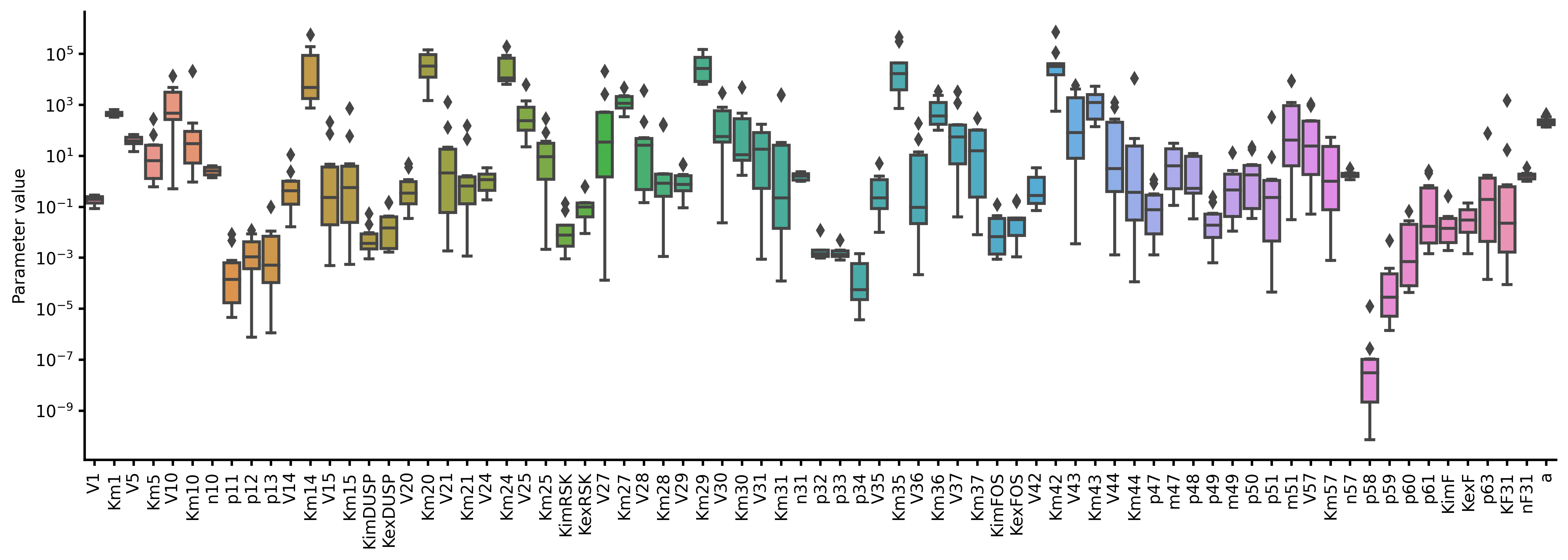
# Visualize estimated parameter sets
res.savefig(figsize=(16,5), boxplot_kws={"orient": "v"})

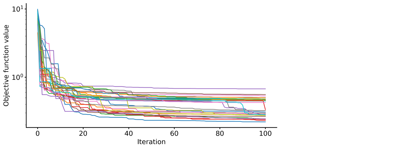
https://raw.githubusercontent.com/biomass-dev/biomass/master/docs/_static/img/estimated_parameter_sets.png

# Visualize objective function traces for different optimization runs.
res.trace_obj()

https://raw.githubusercontent.com/biomass-dev/biomass/master/docs/_static/img/obj_func_trace.png

Visualization of simulation results

from biomass import run_simulation

run_simulation(model, viz_type='average', show_all=False, stdev=True)

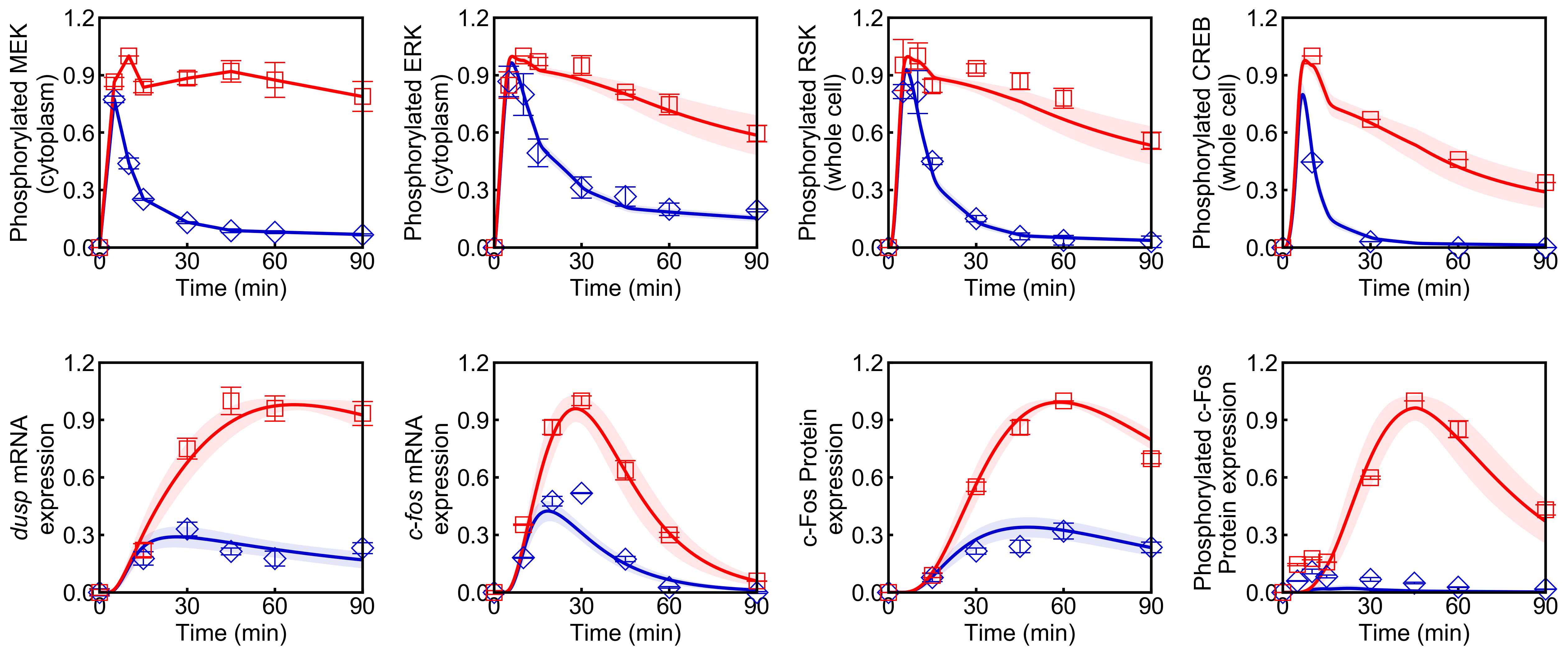
https://raw.githubusercontent.com/biomass-dev/biomass/master/docs/_static/img/simulation_average.png

Points (blue diamonds, EGF; red squares, HRG) denote experimental data, solid lines denote simulations.

Sensitivity analysis

Sensitivity analysis examines how perturbations to the processes in the model affect the quantity of interest, e.g., the integral of the pc-Fos concentration.

To perform sensitivity analysis on reaction rates (target='reaction'), you will need to modify reaction_network.py in the model folder as follows:

class ReactionNetwork(object):

    def __init__(self) -> None:
        """
        Reaction indices grouped according to biological processes.
        This is used for sensitivity analysis (target='reaction').
        """
        super(ReactionNetwork, self).__init__()

        self.reactions: Dict[str, List[int]] = {
            "ERK_activation": [i for i in range(1, 7)],
            "ERK_dephosphorylation_by_DUSP": [i for i in range(47, 57)],
            "ERK_transport": [i for i in range(7, 10)],
            "RSK_activation": [24, 25],
            "RSK_transport": [26],
            "Elk1_activation": [29, 30],
            "CREB_activation": [27, 28],
            "dusp_production_etc": [i for i in range(10, 14)],
            "DUSP_transport": [18, 19],
            "DUSP_stabilization": [14, 15, 20, 21],
            "DUSP_degradation": [16, 17, 22, 23],
            "cfos_production_etc": [i for i in range(31, 35)],
            "cFos_transport": [40, 41],
            "cFos_stabilization": [35, 36, 37, 42, 43, 44],
            "cFos_degradation": [38, 39, 45, 46],
            "Feedback_from_F": [i for i in range(57, 64)],
        }

        ...

Then, run the following code:

from biomass import run_analysis

run_analysis(model, target='reaction', metric='integral', style='barplot', options={'overwrite': True})

The single parameter sensitivity of each reaction is defined by

\[C^{M}_{i} = d \ln{M} / d \ln{v_{i}}\]

where v_i is the i^th reaction rate, v is reaction vector v = (v₁, v₂, …) and M is a signaling metric, e.g., time-integrated response, duration. Sensitivity coefficients are calculated using finite difference approximations with 1% changes in the reaction rates [Kholodenko et al., 1997].

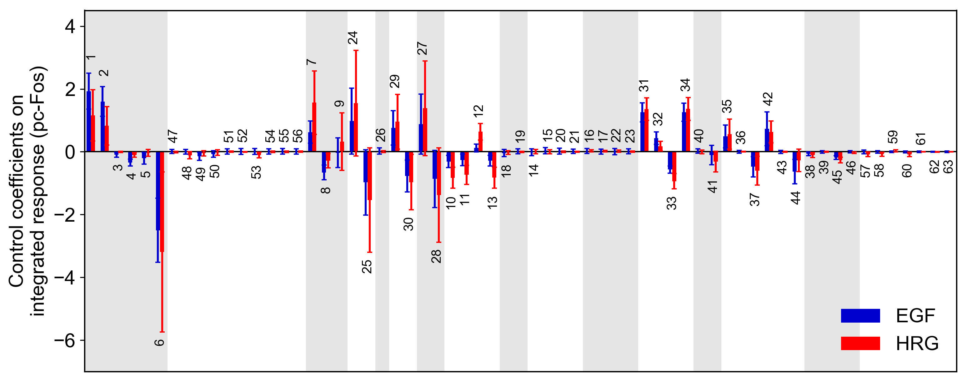
https://raw.githubusercontent.com/biomass-dev/biomass/master/docs/_static/img/sensitivity_PcFos.png

Control coefficients for integrated pc-Fos are shown by bars (blue, EGF; red, HRG). Numbers above bars indicate the reaction indices, and error bars correspond to simulation standard deviation.

Note

If you want to reuse a result from the previous computation and don’t want to calculate sensitivity coefficients again, set options['overwrite'] to False.

Tutorial 1: parameter estimation and sensitivity analysis

Requirements

Model preparation

Prepare a text file describing the biochemical reactions

Set the input of the model

Normalize simulation results

Choose an ODE solver to use

Set experimental data for parameterization of the model

Set lower/upper bounds of parameters to be estimated

Create a new model

Need help?

Parameter estimation

Using optimize() function

Data export and visualization

Visualization of simulation results

Sensitivity analysis

Using `optimize()` function